Making trackpy fast(er)¶

Subnetworks¶

As we’ll see in the examples below, the need to resolve “subnetworks” — in which multiple neighboring particles in one frame could correspond to multiple particles in the next — can drastically slow down tracking. There is a seprate tutorial on dealing with (excessive) subnetworks. In the text below, we’ll look at some methods for finding out just how much a of a problem subnetworks are in your application, so that you can weigh the various remedies against a potential loss of accuracy.

Feature-finding: The best advice¶

Judicious use of the minmass and/or threshold parameters during feature-finding, as described in the “walkthrough” tutorial notebook, can considerably speed up feature-finding, linking, and analysis of tracks. The best way to speed up a computation is usually to avoid doing it at all.

Feature-finding: The details¶

The locate() and batch() functions for feature-finding can use either of two engines for their work, as specified by the optional engine parameter:

• The numba engine is reasonably fast. It is the default when numba is installed (see above).
• The python engine is currently slightly more accurate, but considerably slower.

In addition, both engines do some extra work that you might not always need:

• They iteratively try to refine the position of the feature centroid, for the best possible subpixel accuracy. This can be turned off with the parameter max_iterations=0.
• They compute extra data about the feature, such as its eccentricity. This can be turned off with characterize=False.

Note: Before sacrificing accuracy for performance, it’s best to know objectively how much performance you are gaining. Read on to the Advanced Topics section for information about how to time feature-finding.

Theoretical performance diagnostics: performance_report()¶

trackpy provides an easy way to check whether your system is configured for the best performance. Currently, it reports only whether numba is working.

import trackpy.diag
trackpy.diag.performance_report()

Yes, but could it be faster?
FAST: numba is available and enabled (fast subnets and feature-finding).

Empirical performance diagnostics: Timing and profiling¶

What follows is a crash course in how to evaluate the performance of tracking. The general suggestions given above are good starting points, but they are just that — general suggestions. For your specific application, you need specific data about how long the computation takes, and how the computer is spending its time. This information may help you make your own adjustments to your tracking method, or it may help you when asking the trackpy developers for assistance (chances are we’ll be happy to help!).

You will use these techniques with your own data, but let’s use the data from the “walkthrough” tutorial.

Setup¶

import trackpy as tp
import pims

frames = pims.open('../sample_data/bulk_water/*.png', as_grey=True)

The speed at which we can read images from disk is not something we can hope to improve much, so let’s get that out of the way before we do our tests. Also, we don’t need to use all the frames for this example (though you’re welcome to).

# This gets the image data out of the pims ImageSequence object, and into a good old list in memory.
frames_preload = list(frames[:50])

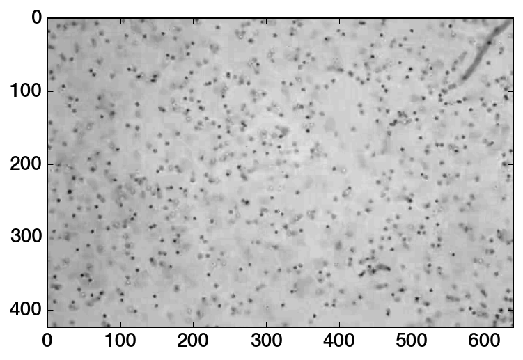
Just so we don’t forget what these images look like:

imshow(frames_preload[0], cmap=matplotlib.cm.gray)

<matplotlib.image.AxesImage at 0x117f48a90>

Before we identify features, we need to give trackpy a chance to “warm up” — initialize fftw and compile certain functions, if it hasn’t done so already. So we’ll find features in just 2 frames:

f2 = tp.batch(frames_preload[:3], 11, minmass=100, invert=True)
_ = tp.batch(frames_preload[:3], 11, minmass=100, invert=True, characterize=False)

Frame 2: 506 features

Timing¶

Let’s find out — precisely — how long it takes to find features in a single frame. You’ll notice that the following cell begins with the line %%timeit. This is an example of a cell magic, which gives IPython special instructions about how to run the rest of the cell.

%%timeit
f1 = tp.batch(frames_preload[:1], 11, minmass=100, invert=True)

Frame 0: 500 features
10 loops, best of 3: 89.7 ms per loop

%%timeit runs the same code multiple times and returns a somewhat accurate measurement of execution time. We can use it to see how much faster we can find features in this image when we turn off centroid refinement and feature characterization:

%%timeit
f1 = tp.batch(frames_preload[:1], 11, minmass=100, invert=True,
              max_iterations=0, characterize=False)

Frame 0: 499 features
10 loops, best of 3: 78.8 ms per loop

One thing to note is that the ratio of features to pixels is rather low in this image. If you were finding features in a dense packing of particles, the timing difference could be much more significant.

Profiling¶

Next, we’ll try to get a sense of what’s taking so long. The %%prun cell magic instructs IPython to run the rest of the cell’s code using a profiler.

%%prun
f = tp.batch(frames_preload, 11, minmass=100, invert=True)

Frame 49: 522 features

When execution is complete, a pager will pop up in the lower portion of the notebook window. This is the profiler output. We reproduce a portion of it here. Your results will depend on your data and the computer you are using.

     123225 function calls (121986 primitive calls) in 4.480 seconds

Ordered by: internal time

ncalls  tottime  percall  cumtime  percall filename:lineno(function)
   50    2.709    0.054    2.709    0.054 {scipy.ndimage._nd_image.min_or_max_filter}
   50    0.481    0.010    0.481    0.010 {scipy.ndimage._nd_image.binary_erosion}
  100    0.299    0.003    0.299    0.003 {scipy.ndimage._nd_image.correlate1d}
  100    0.205    0.002    0.205    0.002 {scipy.ndimage._nd_image.uniform_filter1d}
  100    0.128    0.001    0.128    0.001 {method 'nonzero' of 'numpy.ndarray' objects}
   50    0.079    0.002    0.164    0.003 feature.py:103(refine)
  100    0.078    0.001    0.078    0.001 {numpy.core.multiarray.where}
  100    0.053    0.001    0.053    0.001 {method 'query_pairs' of 'scipy.spatial.ckdtree.cKDTree' objects}
   50    0.036    0.001    0.607    0.012 preprocessing.py:14(bandpass)
   50    0.033    0.001    0.195    0.004 feature.py:27(percentile_threshold)
   50    0.032    0.001    2.989    0.060 feature.py:36(local_maxima)
   50    0.029    0.001    0.526    0.011 uncertainty.py:12(measure_noise)

This is a record of how the computer spent its time while finding features. The various numbers are explained in the documentation for the Python ``profiler` module <http://docs.python.org/2/library/profile.html#instant-user-s-manual>`__. You shouldn’t try to understand every line, but you can get some idea of which functions are called for each frame (multiples of 50), and which are called for each particle. Note that {functions in braces} are written in C, not Python, are not part of trackpy, and tend to be less user-serviceable.

Now let’s look at the linking step. Once again, we’ll prime trackpy, to avoid distorting our results with one-time setup code:

# Use a large search_range, to be sure that numba subnet code is compiled and used.
t1 = tp.link_df(f2, 10, memory=3)

Frame 2: 506 trajectories present

%%prun
t = tp.link_df(f, 5, memory=3)

Frame 49: 522 trajectories present

     770140 function calls (766921 primitive calls) in 1.652 seconds

Ordered by: internal time

ncalls  tottime  percall  cumtime  percall filename:lineno(function)
   51    0.229    0.004    1.180    0.023 linking.py:926(link)
  149    0.140    0.001    0.322    0.002 {map}
28925/28825    0.096    0.000    0.099    0.000 {numpy.core.multiarray.array}
   49    0.082    0.002    0.240    0.005 linking.py:1182(assign_candidates)
   49    0.077    0.002    0.080    0.002 {method 'query' of 'scipy.spatial.ckdtree.cKDTree' objects}
   49    0.073    0.001    0.118    0.002 linking.py:1069(_assign_links)
25945    0.064    0.000    0.179    0.000 linking.py:368(__init__)
27415    0.048    0.000    0.117    0.000 numeric.py:394(asarray)
25945    0.042    0.000    0.042    0.000 linking.py:300(__init__)
54280    0.040    0.000    0.051    0.000 {method 'sort' of 'list' objects}
   50    0.039    0.001    0.039    0.001 {pandas.lib.clean_index_list}
    1    0.037    0.037    1.652    1.652 linking.py:470(link_df)
   98    0.031    0.000    0.097    0.001 linking.py:32(rebuild)
  300    0.024    0.000    0.043    0.000 common.py:303(_isnull_ndarraylike)
54115    0.022    0.000    0.022    0.000 linking.py:345(track)
54280    0.021    0.000    0.021    0.000 linking.py:47(<lambda>)
  101    0.021    0.000    0.021    0.000 {method 'get_indexer' of 'pandas.index.IndexEngine' objects}
112445    0.018    0.000    0.018    0.000 {method 'append' of 'list' objects}
 1265    0.018    0.000    0.018    0.000 {method 'reduce' of 'numpy.ufunc' objects}
25945    0.018    0.000    0.030    0.000 linking.py:196(add_point)
89361/86242    0.017    0.000    0.019    0.000 {len}
  136    0.016    0.000    0.021    0.000 linking.py:1375(numba_link)

This goes much faster than feature identification, though to be fair, we have far, far more pixels than particles. Note the calls to numba_link at the end of the report; this is the subnet resolution code referred to above. If you require a large search_range, these computations can dramatically slow down linking. As it is, they are under control.

pyfftw and the frequency-domain bandpass¶

trackpy performs bandpass filtering to prepare an image for feature-finding. As of version 0.3, this is done with convolution; formerly, it was done using fast Fourier transforms (FFT). The two methods yield very close results, but the convolution method is roughly twice as fast.

Because the two methods are not mathematically identical, trackpy still includes the FFT method in case you would like to use it (or just compare its results). This method is not available as part of locate(); you must perform the bandpass separately and then call locate() with preprocess=False. You can perform the FFT bandpass with one of two functions:

• trackpy.preprocessing.legacy_bandpass() uses the FFT functions built into numpy.
• trackpy.preprocessing.legacy_bandpass_fftw() uses the FFTW library, an exceptionally fast implementation of FFT. pyfftw is the module that lets Python programs use it. Like numba it is optional, but it can speed up the bandpass operation by a factor of ~3. (The default method now in trackpy is faster still.)

You should be able to install FFTW from your Linux package manager, or on the Mac using Homebrew (with the command brew install fftw). Once you’ve done that, pyfftw itself should install with pip install pyfftw

Neighbor-finding strategy: KDTree¶

An important operation in tracking (i.e. linking) is finding all the particles that are close to a certain point in space. trackpy has two ways of doing this:

• A KDTree, which only handles more standard cases (e.g. Euclidean geometries) and is written in C. (This is the default.)
• A hash table written in pure Python. It is very extensible but tends to be slower.

The method is set by the neighbor_strategy argument to the various linking functions, which again defaults to KDTree. The KDTree is a standard part of scipy; if you can run trackpy at all, it is enabled.

Well, I hope you’ve enjoyed this brief tour of trackpy performance. Just remember that if you come up with new ways to improve performance, the trackpy community will be interested!